Building an Automated Image Captioning Application

Note: You can get the source code on the project’s repository.

Background

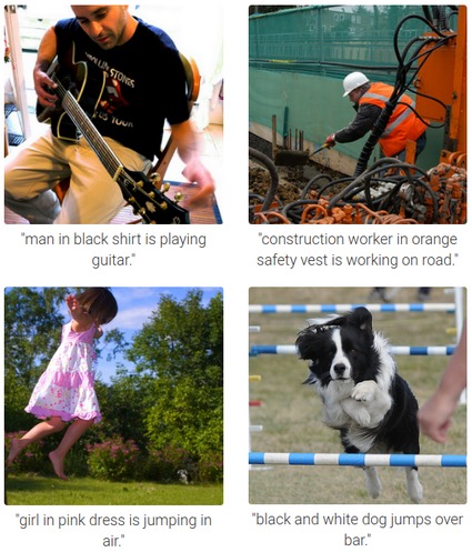
In 2016 I found an intriguing paper by Karpathy et al. about automated image captioning. I had never thought AI would arrive at this stage that fast. Some examples presented in the paper was horrifyingly accurate and detailed:

Aware that it’s deep learning that made this breakthrough possible, I did a research to find the best resource for me to grok deep learning. I finally found Stanford’s CS231n course which was lectured also by Karpathy. I highly recommend to watch its lecture videos and read its lecture notes for anyone who wants to seriously get started with deep learning!

My deep learning exploration continued by reading some chapters of Deep Learning book and many articles / papers recommended at r/MachineLearning. A paper by Vinyals et al. particularly interested me since their model was relatively simpler than Karpathy’s, but their model outperformed it.

I decided to apply my knowledge about deep learning so far by reimplementing Vinyals’ paper. In early 2017 I started the project as a capstone project of a course I was taking. I learned a ton from this project, from learning how to use Keras and TensorFlow, understanding Keras’ internals, troubleshooting Python’s weird process signal handling, building a machine learning model, until the most time consuming one: debugging a machine learning application. In this post I will expound on my exact thought process while I was doing the project.

Note: On some concepts I will only explain the general idea to make sense of it, but I will not go into detail. However, I will provide some links that I think the best resources to learn the concepts.

Sneak Peek

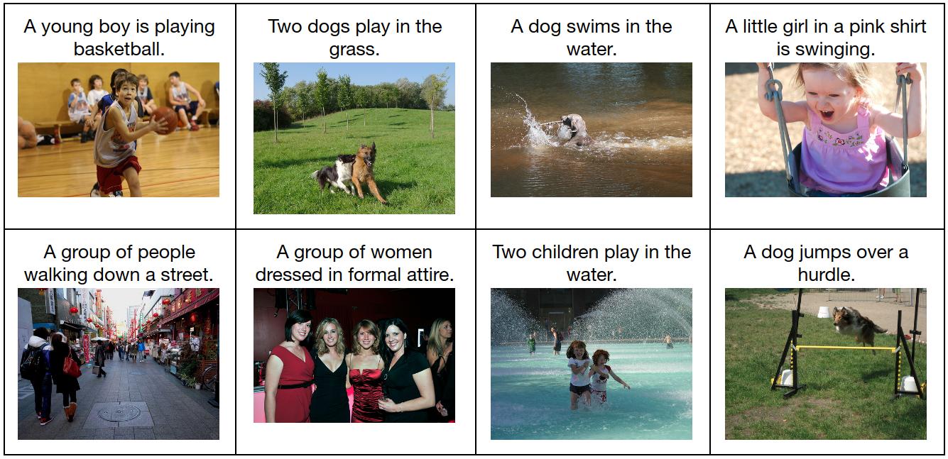
Before we start, I want to show you the performance of the model we will build to give you an idea of what you would expect by the end of the tutorial. As you can see, our model can generate a caption without errors for some images below:

Quantitatively, on Flickr8k dataset our model outperforms Karpathy’s in all metrics below:

Metric	Our Model	Karpathy’s
BLEU-1	61.8	57.9
BLEU-2	40.8	38.3
BLEU-3	27.8	24.5
BLEU-4	19.0	16.0
METEOR	21.5	16.7
CIDEr	41.5	31.8

Learn more: You don’t need to worry if you don’t understand the metrics above. Basically, they assess a generated caption by comparing it to the reference / original caption(s). Curious readers can read this paper for more information.

At the end of tutorial more result examples (including incorrect captions) will be presented and we will compare our model to the original Vinyals’ model.

Flickr8k Dataset

We will use Flickr8k dataset to train our machine learning model. You can request to download the dataset by filling this form. Although many other image captioning datasets (Flickr30k, COCO) are available, Flickr8k is chosen because it takes only a few hours of training on GPU to produce a good model.

The dataset contains 8000 of images each of which has 5 captions by different people. Having more than one caption for each image is desirable because an image can be described in many ways. For example, look an image of Flickr8k below:

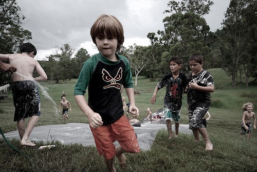
The image above is given 5 different captions:

1. A boy runs as others play on a home-made slip and slide.
2. Children in swimming clothes in a field.
3. Little kids are playing outside with a water hose and are sliding down a water slide.
4. Several children are playing outside with a wet tarp on the ground.
5. Several children playing on a homemade water slide.

As we can see, there are some differences among them:

• Caption 1 focuses on a boy running.
• “Children” vs “kids”.
• Caption 2 is not a grammatically correct sentence.

Having different captions helps a model catch these subtleties and be able to generalize better.

Those 8000 images are divided into 3 sets:

1. Training set (6000 images): We use it for training our model.
2. Validation set (1000 images): We use it for assessing our model’s performance while training.
3. Test set (1000 images): We use it for assessing our model’s performance after training.

Before you continue: You may want to setup the development environment needed (libraries and such) by following the steps on the project’s repository. However, I recommend you read the whole tutorial first to understand the concepts and the ideas. After that you can setup the environment and run a training.

Note: The purpose of every code snippet in this post is to give you a sense on how to implement the concepts explained before. The snippet is a simplified version of a part of methods and/or classes whose location is always linked at the top. You are encouraged to skim (at least) the Python file linked in order to understand how classes and methods in the whole codebase are related to each other. You can see a list of all Python files in the codebase here.

Data Preprocessing

Image Preprocessing

We need to convert an image into a 3-dimensional (height, width, color channel) vector before we can feed it into any machine learning model. We can use some functions provided by Keras to do that:

# A simplified version of https://github.com/danieljl/keras-image-captioning/blob/master/keras_image_captioning/preprocessors.py#L39-L46

from keras.applications import inception_v3
from keras.preprocessing.image import img_to_array, load_img

img_path = "..."
img = load_img(img_path, target_size=(299, 299))
img_array = img_to_array(img)
img_array = inception_v3.preprocess_input(img_array)

We need to resize the image into 299 x 299 pixels in order to match the model’s architecture we will build. img_array would have a shape of (299, 299, 3). The last line simply scales the pixel values into a range of [-1, 1].

Caption Preprocessing

Since machine learning works on numbers only, we need to convert words into numbers. Suppose we have a sentence He has a pen and a book.. We can encode it as integers by 1) converting all words into lower case, 2) removing all punctuations, 3) appending a special end-of-sentence word (EOS), 4) sorting all unique words, and 5) assigning each word with a number:

a = 1
and = 2
book = 3
eos = 4
has = 5
he = 6
pen = 7

After we have this mapping, we can convert the sentence into a list of integers [6, 5, 1, 7, 2, 1, 3, 4]. Again, Keras enables us to implement the conversion in just a few lines of code:

# A simplified version of https://github.com/danieljl/keras-image-captioning/blob/master/keras_image_captioning/preprocessors.py#L82-L90

from keras.preprocessing.text import Tokenizer

all_sentences = ['A dog is sleeping.','A child is running.', 'She is cooking.']
tokenizer = Tokenizer()
# All possible words should be fit first
tokenizer.fit_on_texts(all_sentences)

# Encode first two sentences
sentences_to_encode = all_sentences[:2]
encoded_sentences = tokenizer.texts_to_sequences(sentences_to_encode)

Notice that tokenizer.text_to_sequences method receives a list of sentences and returns a list of lists of integers.

Image Captioning Model Architecture

We will build a model based on deep learning which is just a fancy name of neural networks. There are many types of neural networks, but here we only use three: fully-connected neural networks (FC), convolutional neural networks (CNN), and recurrent neural networks (RNN). FC is just a basic neural network, while the two others have specific purposes. CNN is usually used in image data to capture spatial invariance. RNN is usually used to model sequential data (time series, sentences).

Actually, CNN and RNN are families of neural networks. We will use Inception v3 and LSTM as our CNN and RNN respectively.

Our model is largely based on Vinyals et al. with a few differences:

• For CNN we use Inception v3 instead of Inception v1.
• For RNN we use multi-layered LSTM instead of single-layered one.
• We don’t have a special start-of-sentence word so we feed the first word at $t = 1$ instead of $t = 2$.
• We use different values for some hyperparameters, such as learning rate, dropout rate, embedding size, LSTM output size, and the number of LSTM layers.

Problem Statement

The problem statement we want to solve is: Given an image, find the most probable sequence of words (sentence) describing the image. Fortunately, a deep learning model can be trained by directly maximizing the probability of the correct description given the image. In the training phase we want to find the best model’s parameters $\theta^*$ which satisfies:

$$\theta^* = \arg \max_{\theta} \sum_{(I, S)} \log p(S \mid I; \theta)$$

where $\theta$ are the parameters of our model, $I$ is an image, and $S$ is its correct caption.

The probability of the correct caption $S$ given an image $I$ can be modeled as the joint probability over its words $S_0, \dots, S_N$:

$$\log p(S \mid I) = \sum_{t = 0}^N \log p_t(S_t \mid I, S_0, \dots, S_{t - 1})$$

where $N$ is the length of caption $S$, $S_N$ is a special end-of-sentence word (EOS), and the relationship between $S$ and $S_i$ is defined by:

$$S = \mathrm{Concatenate}(S_0, S_1, \dots, S_N)$$

We can use LSTM to model the joint probability distribution. Before that we need to encode images and captions into fixed-length dimensional vectors.

Image Embeddings

We can think of a CNN as an automatic feature extractor. At the first few layers we expect a CNN to generate low-level features, such as lines and arcs. The next few layers transforms these low-level features into higher-level features, such as shapes. This continues until the last layer where we expect the CNN will generate high-level enough features (e.g. objects) that can be fed into another type of neural network.

In Inception v3 that type of neural network is an FC because it was initially designed for solving image classification problems (ImageNet) where the image labels are predefined. The output size of the FC is the number of ImageNet labels (1000).

In image captioning problem we cannot do that since we are not given some predefined captions. Our model is expected to caption an image solely based on the image itself and the vocabulary of unique words in the training set. You might think we could enumerate all possible captions from the vocabulary. It’s not feasible as the number of possibilities would be $\text{unique-words} ^ \text{sentence-length}$.

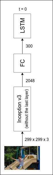
Since LSTM can model the probability of the correct caption given an image, a better approach would be feeding the result of Inception v3 (without its last FC layer) into an LSTM. The input size of the LSTM is not necessarily the same as the output size of the Inception v3, so using an FC we first transform that output into some fixed-length (300) dimensional vectors which are called image embeddings.

The complete diagram of image embedding architecture is shown below. Remember that in Image Preprocessing section we’ve transformed images into 3-dimensional vectors of shape of (299, 299, 3) to match Inception v3’s input size.

We can implement the architecture above (without LSTM yet) as below. Notice that we don’t train Inception v3 from scratch. Instead, we use and fix weights from a training on ImageNet dataset. This is called transfer learning.

Before you continue: If you are new to Keras, you may want to read first this official tutorial on how to build a model.

# A simplified version of https://github.com/danieljl/keras-image-captioning/blob/master/keras_image_captioning/models.py#L105-L120

from keras.applications.inception_v3 import InceptionV3
from keras.layers import BatchNormalization, Dense, RepeatVector

# The top layer is the last layer
image_model = InceptionV3(include_top=False, weights='imagenet', pooling='avg')
# Fix the weights
for layer in image_model.layers:
  layer.trainable = False

embedding_size = 300
dense_input = BatchNormalization(axis=-1)(image_model.output)
image_dense = Dense(units=embedding_size)(dense_input)  # FC layer
# Add a timestep dimension to match LSTM's input size
image_embedding = RepeatVector(1)(image_dense)
image_input = image_model.input

# image_input and image_embedding will be used by another following snippet

Learn more: Batch normalization is a technique to accelerate deep learning training. Curious readers can read the original paper.

Word Embeddings

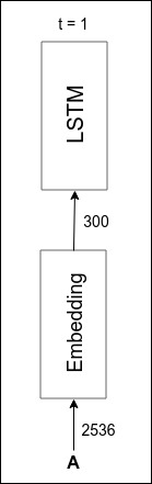
In Caption Processing section we’ve transformed words into integers. Similar to images, words have to be converted into some fixed-length (300) dimensional vectors before they can be fed into LSTM. It can be achieved by two simple steps:

1. Encode the integers representing words using one-hot encoding into some fixed-length vectors. Suppose the total number of unique words is 5 and we have a word encoded as an integer of 2. The one-hot encoding of it would be [0, 0, 1, 0, 0]. Notice that the word is turned into a vector whose dimension equals to the total number of unique words.
2. We can now transform the one-hot-encoded vectors into 300-dimensional vectors using an FC (Dense layer in Keras). The input size would be the total number of unique words and the output size would be 300. These output vectors are called word embeddings.

The complete diagram of image embedding architecture is shown below:

An implementation (without LSTM yet) in Keras could be simpler as Keras provides another type of layer called Embedding which does exactly the two steps above:

# A simplified version of https://github.com/danieljl/keras-image-captioning/blob/master/keras_image_captioning/models.py#L122-L140

from keras.layers import Embedding, Input

vocab_size = 2536
embedding_size = 300
sentence_input = Input(shape=[None])
word_embedding = Embedding(input_dim=vocab_size,
                           output_dim=embedding_size
                           )(sentence_input)

# sentence_input and word_embedding will be used in another following snippet

Sequence Model

Now we have turned images and captions into embedding vectors, but there is another question remaining: how these vectors are fed as inputs to the LSTM.

Remember the joint probability formula in Problem Statement section:

$$\log p(S \mid I) = \sum_{t = 0}^N \log p_t(S_t \mid I, S_0, \dots, S_{t - 1})$$

We also define $\mathrm{LSTM}_i$ as the LSTM’s output at timestep $t = i$. (Well, the definition is not entirely correct. It will be redefined soon.)

Using an LSTM we can model the joint probability distribution such that:

$$\mathrm{LSTM}_i = p_i$$

In order to achieve that, at the training phase we feed:

1. the image embedding as the LSTM’s input at $t = 0$,
2. the 0-th word embedding as the LSTM’s input at $t = 1$,
3. and so on until the last word embedding.

Details about the LSTM model:

• Its output size is set to 300, which is the same as the embedding’s size.
• The number of LSTM layers is set to 3.
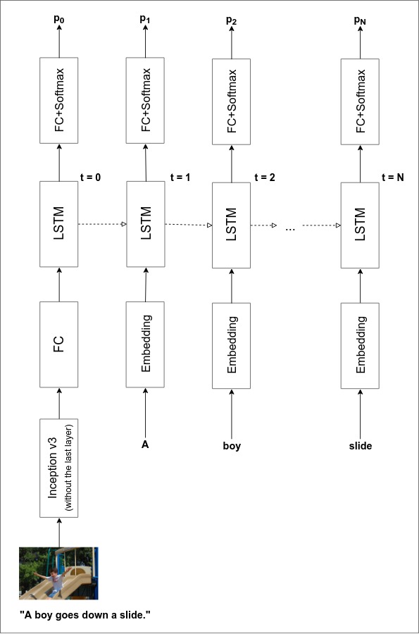
• Since we need the LSTM to model the probability distribution $p_i$ over all words, after LSTM layer we put an FC layer whose output size matches the vocabulary’s size. So, the correct definition of $\mathrm{LSTM}_i$ is actually the output of this FC layer.

The complete model architecture is as shown below. While we stack three layers of LSTM, the diagram shows only one for simplicity.

Now we can continue the implementation by feeding the embeddings into the LSTM. Learning rate, optimizer, loss, and metrics will be discussed in the next section.

# A simplified version of these two:
#   - https://github.com/danieljl/keras-image-captioning/blob/master/keras_image_captioning/models.py#L85-L103
#   - https://github.com/danieljl/keras-image-captioning/blob/master/keras_image_captioning/models.py#L142-L163

# image_input, image_embedding, sentence_input, and word_embedding are
# the same variables as the ones in the previous code snippets

from keras.layers import (BatchNormalization, Concatenate, Dense, LSTM,
                          TimeDistributed)
from keras.models import Model
from keras.optimizers import Adam

sequence_input = Concatenate(axis=1)([image_embedding, word_embedding])

learning_rate = 0.00051
lstm_output_size = 300
vocab_size = 2536
lstm_layers = 3
dropout_rate = 0.22
input_ = sequence_input

for _ in range(lstm_layers):
  input_ = BatchNormalization(axis=-1)(input_)
  lstm_out = LSTM(units=lstm_output_size,
                  return_sequences=True,
                  dropout=dropout_rate,
                  recurrent_dropout=dropout_rate)(input_)
  input_ = lstm_out
sequence_output = TimeDistributed(Dense(units=vocab_size))(lstm_out)

model = Model(inputs=[image_input, sentence_input],
              outputs=sequence_output)
model.compile(optimizer=Adam(lr=learning_rate),
              loss=categorical_crossentropy_from_logits,
              metrics=[categorical_accuracy_with_variable_timestep])

# model will be used in another following snippet

Learn more: Dropout is a commonly used regularization technique in neural networks. Curious readers can read more about it in CS231n’s lecture notes or the original paper.

Training Phase

Loss Function

One crucial step to do before we can train the model is to define a loss function. Since $\mathrm{LSTM}_i = p_i$ represents a probability distribution over all words, we can think of it as a multiclass classification where the number of classes equals the vocabulary’s size. Therefore, we can use a commonly used loss function for multiclass classification problems: cross-entropy loss. The only difference is we need to aggregate all losses over the whole timesteps:

$$L(I, S) = - \sum_{t = 0}^N \log p_t(S_t)$$

where $p_t(S_t)$ represents the probability of word $S_t$ in distribution $p_t$.

In the codebase EOS is unnecessarily fed into the model so we have to discard timestep $t = N + 1$ when calculating the loss:

# Taken from https://github.com/danieljl/keras-image-captioning/blob/master/keras_image_captioning/losses.py

import tensorflow as tf

def categorical_crossentropy_from_logits(y_true, y_pred):
  y_true = y_true[:, :-1, :]  # Discard the last timestep
  y_pred = y_pred[:, :-1, :]  # Discard the last timestep
  loss = tf.nn.softmax_cross_entropy_with_logits(labels=y_true,
                                                 logits=y_pred)
  return loss

Metric

Similarly, we can use a commonly used metric for multiclass classification: categorical accuracy. Again, we need to aggregate all the values over the whole timesteps:

# Taken from https://github.com/danieljl/keras-image-captioning/blob/master/keras_image_captioning/metrics.py#L78-L99

import tensorflow as tf

def categorical_accuracy_with_variable_timestep(y_true, y_pred):
  y_true = y_true[:, :-1, :]  # Discard the last timestep
  y_pred = y_pred[:, :-1, :]  # Discard the last timestep

  # Flatten the timestep dimension
  shape = tf.shape(y_true)
  y_true = tf.reshape(y_true, [-1, shape[-1]])
  y_pred = tf.reshape(y_pred, [-1, shape[-1]])

  # Discard rows that are all zeros as they represent padding words.
  is_zero_y_true = tf.equal(y_true, 0)
  is_zero_row_y_true = tf.reduce_all(is_zero_y_true, axis=-1)
  y_true = tf.boolean_mask(y_true, ~is_zero_row_y_true)
  y_pred = tf.boolean_mask(y_pred, ~is_zero_row_y_true)

  accuracy = tf.reduce_mean(tf.cast(tf.equal(tf.argmax(y_true, axis=1),
                                              tf.argmax(y_pred, axis=1)),
                                    dtype=tf.float32))
  return accuracy

You might think that categorical accuracy is not a good metric for image captioning problems since if the model produces a very similar caption to the correct one but is not arranged with it, the accuracy will be very low. The better metrics would be BLEU, METEOR, and CIDEr which were mentioned before in Sneak Peek section.

You are right. However, those metrics are computationally expensive because of the need of inference. Although categorical accuracy is not very accurate in assessing the model, the fact that it is quite correlated with those metrics makes it reasonable to use in the training phase.

Optimization

We will train our model by minimizing the loss function using an optimization method called stochastic gradient descent (SGD). Specifically, we will use Adam, a variant of SGD, which makes the training converge faster than a vanilla SGD does. The learning rate is set to 0.00051.

To minimize the loss, the optimizer needs the gradient of the loss function which tells the optimizer how much and in which direction it needs to adjust each model’s parameter. The famous backpropagation is an efficient method to calculate the gradient of neural networks.

Batch Training

So far we only discuss a training on a single example. We can do a full training by applying the SGD over the whole training set repeatedly until it converges. For performance reasons, typically we apply the SGD on a batch of examples instead of a single example.

Due to batches, we need to append some captions with “padding words” in order that captions within a batch have the same length. These padding words have to be encoded in such a way they won’t increase the loss. The trick is to encode them in one-hot encoding where all values are zeros.

Suppose the vocabulary size is 3 and we have a batch of captions [[1, 2, 0], [1, 0]]. Its one-hot encoding would be:

# before padding:
[[[0, 1, 0],
  [0, 0, 1],
  [1, 0, 0]],
 [[0, 1, 0],
  [1, 0, 0]]]

# after padding:
[[[0, 1, 0],
  [0, 0, 1],
  [1, 0, 0]],
 [[0, 1, 0],
  [1, 0, 0],
  [0, 0, 0]]]  # padding

At last, we can run a training by calling Keras’ Model.fit_generator as below. DatasetProvider is a class which generates batches with a help from Flickr8kDataset, ImagePreprocessor, and CaptionPreprocessor.

# A simplified version of https://github.com/danieljl/keras-image-captioning/blob/master/keras_image_captioning/training.py#L84-L112

# DatasetProvider's source: https://github.com/danieljl/keras-image-captioning/blob/master/keras_image_captioning/dataset_providers.py#L13-L128
from keras_image_captioning.dataset_providers import DatasetProvider

dataset_provider = DatasetProvider()
epochs = 33  # the number of passes through the entire training set

# model is the same variable as the one in the previous code snippet
model.fit_generator(generator=dataset_provider.training_set(),
                    steps_per_epoch=dataset_provider.training_steps,
                    epochs=epochs,
                    validation_data=dataset_provider.validation_set(),
                    validation_steps=dataset_provider.validation_steps)

Inference Phase

At the inference phase we expect the model to generate the most probable caption $S^*$ given an image $I$. In a mathematical form, it can be written as:

$$\begin{align} S^* & = \arg \max_S \log p(S \mid I) \\ & = \arg \max_S \sum_{t = 0}^N \log p_t(S_t \mid I, S_0, \dots, S_{t - 1}) \\ & = \arg \max_S \sum_{t = 0}^N \log \mathrm{LSTM}_t(S_t \mid I, S_0, \dots, S_{t - 1}) \\ \end{align}$$

One way to do it is by following these steps:

1. Feed the image into the Image Embedding Model which will produce an image embedding of the image.
2. The image embedding will be the input for the Sequence Model (LSTM) at timestep $t = 0$. It will yield the probability distribution of the first word.
3. Choose the first word by selecting the word with the highest probability in that distribution.
4. Feed this first generated word into the Word Embedding Model which will produce a word embedding of the first word.
5. The word embedding will be the input for the Sequence Model (LSTM) at timestep $t = 1$. It will yield the probability distribution of the second word.
6. Repeat a similar process (3 - 5) until the end-of-sentence word (EOS) is generated or the maximum of length is reached.

You may notice that the algorithm above is a greedy approach to approximate $S^*$ since we consider only the most probable word at each timestep (step 3 above). Despite that, we cannot calculate $S^*$ by considering all words in the vocabulary since the time complexity will be exponential to the caption’s length.

Beam Search

A better approach would be in the middle, i.e. by considering the top $M$ most probable words at each timestep. It is still exponential though, so we can make it linear by only taking $M$ partial captions to the next timestep. This approach is called beam search.

Before describing a pseudocode of beam search, we define $R_t$ as a partial caption until $t$ -th word:

$$R_t = \mathrm{Concatenate}(S_0, S_1, \dots, S_t)$$

Therefore, the log probability distribution of a partial caption $R_t$ given an image $I$ is:

$$\begin{align} \log p(R_t \mid I) & = \sum_{u = 0}^t \log p_u(S_u \mid I, S_0, \dots, S_{u - 1}) \\ & = \log p(R_{t - 1} \mid I) + \log p_t(S_t \mid I, S_0, \dots, S_{t - 1}) \\ & = \log p(R_{t - 1} \mid I) + \log p_t(S_t \mid I, R_{t - 1}) \\ & = \log p(R_{t - 1} \mid I) + \log \mathrm{LSTM}_t(S_t \mid I, R_{t - 1}) \end{align}$$

A pseudocode of beam search for our problem is relatively simple:

1. While below the maximum of caption’s length, do:

   1. For each partial caption $R_{t - 1}$ in the top $M$ partial captions of the previous timestep $t - 1$:

      1. Run an inference with this partial caption $R_{t - 1}$. It will produce the probability distribution of the next word $S_t$ given the image $I$ and the partial caption $R_{t - 1}$:

         $$p_t(S_t \mid I, R_{t - 1}) = \mathrm{LSTM}_t(S_t \mid I, R_{t - 1})$$

      2. Calculate the log probability distribution of a partial caption $R_t$ given an image $I$. Note that we have $\log p(R_{t - 1} \mid I)$ from the previous iteration.

         $$\begin{align} \log p(R_t \mid I) & = \log p(R_{t - 1} \mid I) \\ & + \log \mathrm{LSTM}_t(S_t \mid I, R_{t - 1}) \end{align}$$

      3. Choose the top $M$ partial captions in the $p(R_t \mid I)$ distribution.

   2. Choose top $M$ partial captions out of all the top $M \times M$ partial captions from all for-each iterations before.

As in the training phase, for performance reasons we have to implement beam search to handle batches. It becomes more complicated than I’ve ever thought. Curious readers can read the implementation of BeamSearchInference here.

Model’s Performance

In the Sneak Peek section we’ve seen a glance of our model’s performance. We will discuss it more in this section.

When assessing a machine learning model, we want to measure its generalization performance, that is, we want know how it performs on examples which haven’t been seen before. These examples are called a test set. Flickr8k dataset has a test set of 1000 examples which we will use to assess our model.

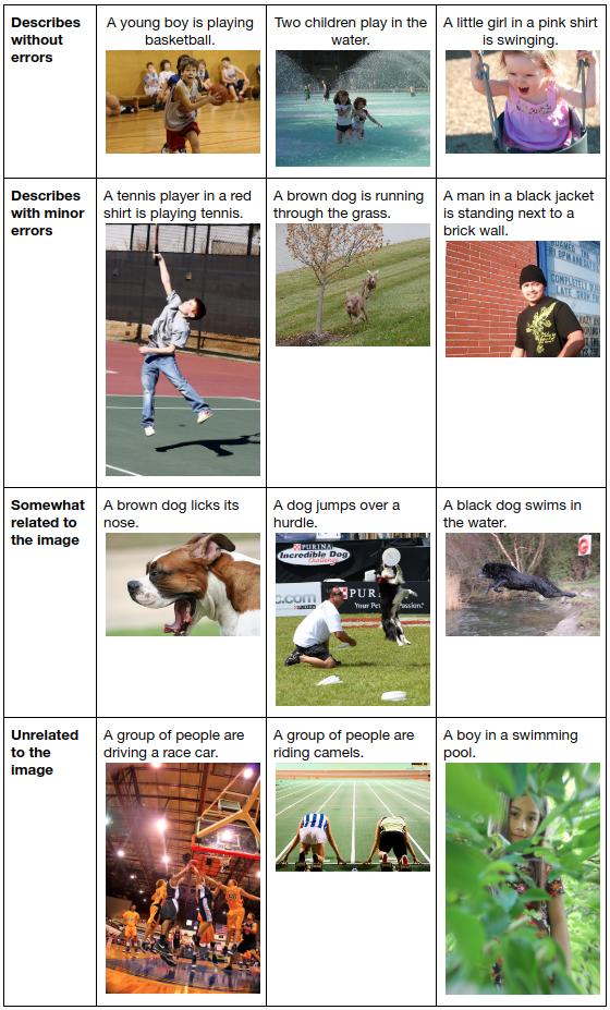
Qualitative Assessment

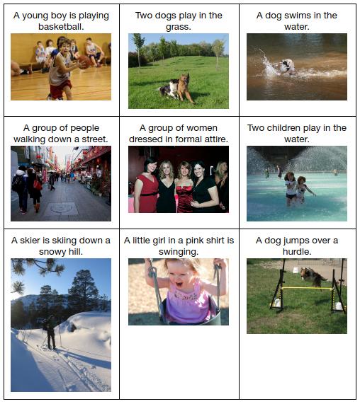
As we can see below, the captions generated by our model ranging from “describes without errors” to “unrelated to the image”:

Quantitative Assessment

BLUE, METEOR, and CIDEr are quantitative metrics commonly used in image captioning problems. Basically, they assess a generated caption by comparing it to the reference caption(s). You can read more about them in this paper.

As shown in the table below, our model’s performance is on par with the original Vinyals’ model. We’ve successfully reproduced the result from the paper! Compare to Karpathy’s model, our model outperforms it in all metrics.

Metric	Our Model	Vinyals’	Karpathy’s
BLEU-1	61.8	63	57.9
BLEU-2	40.8	41	38.3
BLEU-3	27.8	27	24.5
BLEU-4	19.0	N/A	16.0
METEOR	21.5	N/A	16.7
CIDEr	41.5	N/A	31.8

Hyperparameters

You might have been wondering why we set dropout rate, embedding size, LSTM output size, learning rate, and the number of LSTM layers to such values. These come from the hyperparameter search I’ve done before using a technique proposed by Bergstra et al.. We don’t use the values proposed by Vinyals et al. since in the experiment I found they are inferior to the values from the hyperparameter search.

To recap, the table below shows the hyperparameters of our model:

Hyperparameter	Value
Learning rate	0.00051
Batch size	32
Epochs	33
Dropout rate	0.22
Embedding size	300
LSTM output size	300
LSTM layers	3

Epilogue

You can setup the development environment, run a training, and run an inference with just a few lines of commands by following the steps in the project’s repository. All snippets in this post are just simplified versions of the codebase. Also, there are so many parts of the codebase that are not shown in this post. You may want to read or skim the whole codebase to understand how classes and methods in the whole codebase are related to each other.

My tip for reading any code is to read a method together with its unit test. That way you will understand how the method is called, what input or precondition it requires, and what output or postcondition you would expect the method will produce. Fortunately, almost every method in the codebase has a unit test.

Happy learning!